Lab 3: ToF Sensors
02.11.2025 - 02.25.2025
Setup
The objective of Lab 3 was to configure the time of flight sensors, which measure distance to aid with obstacle detection and navigation. Lab tasks included soldering components to the Artemis and analyzing data and communication speed.
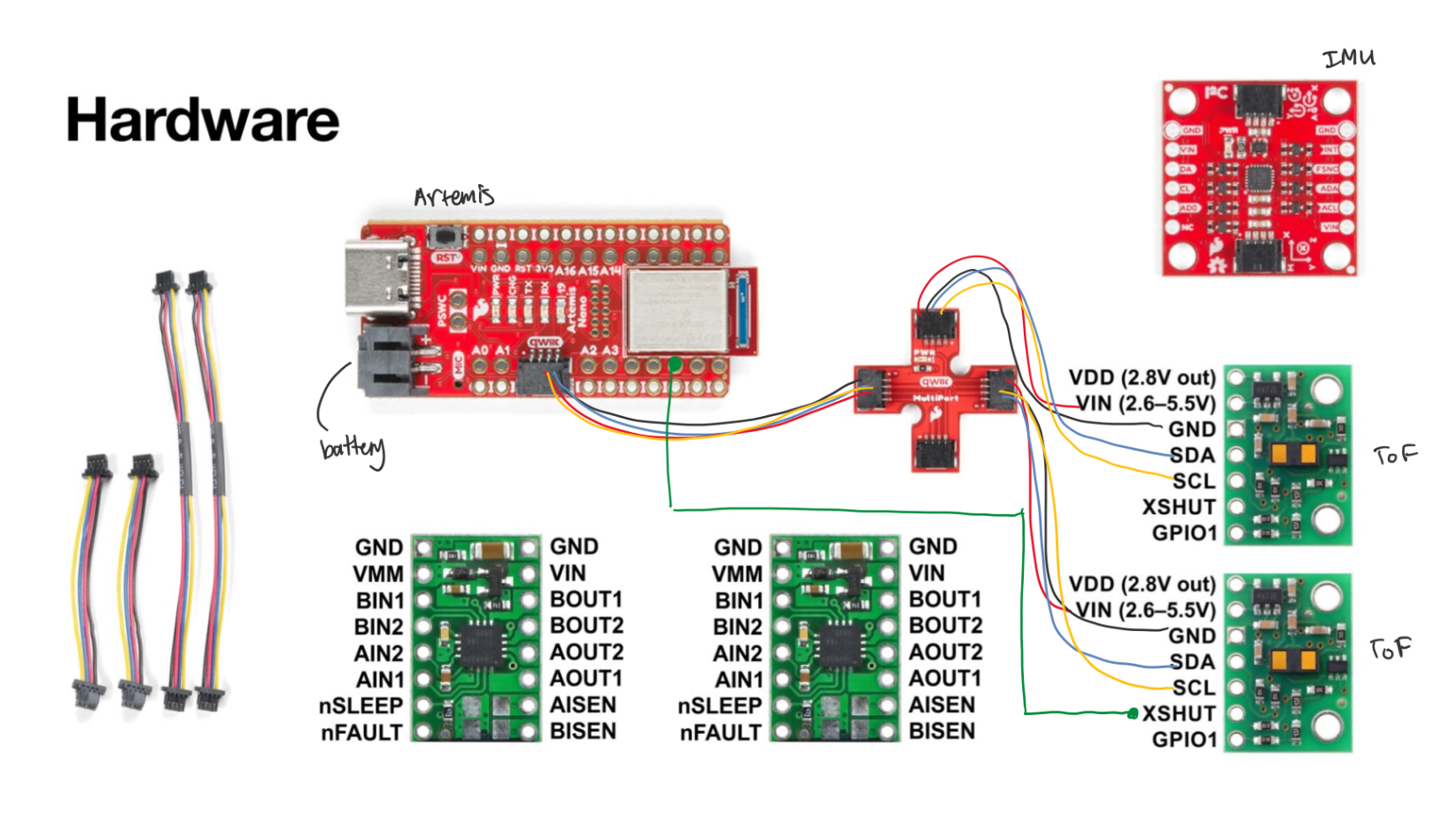
Before beginning the lab, I planned out how I was going to wire the components together, which can be seen in the figure above. I decided to place one ToF sensor on the front of the car, and the other on the side of the car. This would be helpful when detecting obstacles, as this placement would allow the robot to see in front and to the side. Because we are using two ToF sensors, they will have the same I2C address by default. In order to measure data using both of the sensors, I used the XSHUT pin on one of the sensors in order to temporarily shut off one of the sensors and change the I2C address of the other.
Soldering
In this lab, I had to solder a connector to the battery, two QWIIC connectors to the ToF sensors, and the XSHUT pin of one of the sensors to one of the GPIO pins on the Artemis.
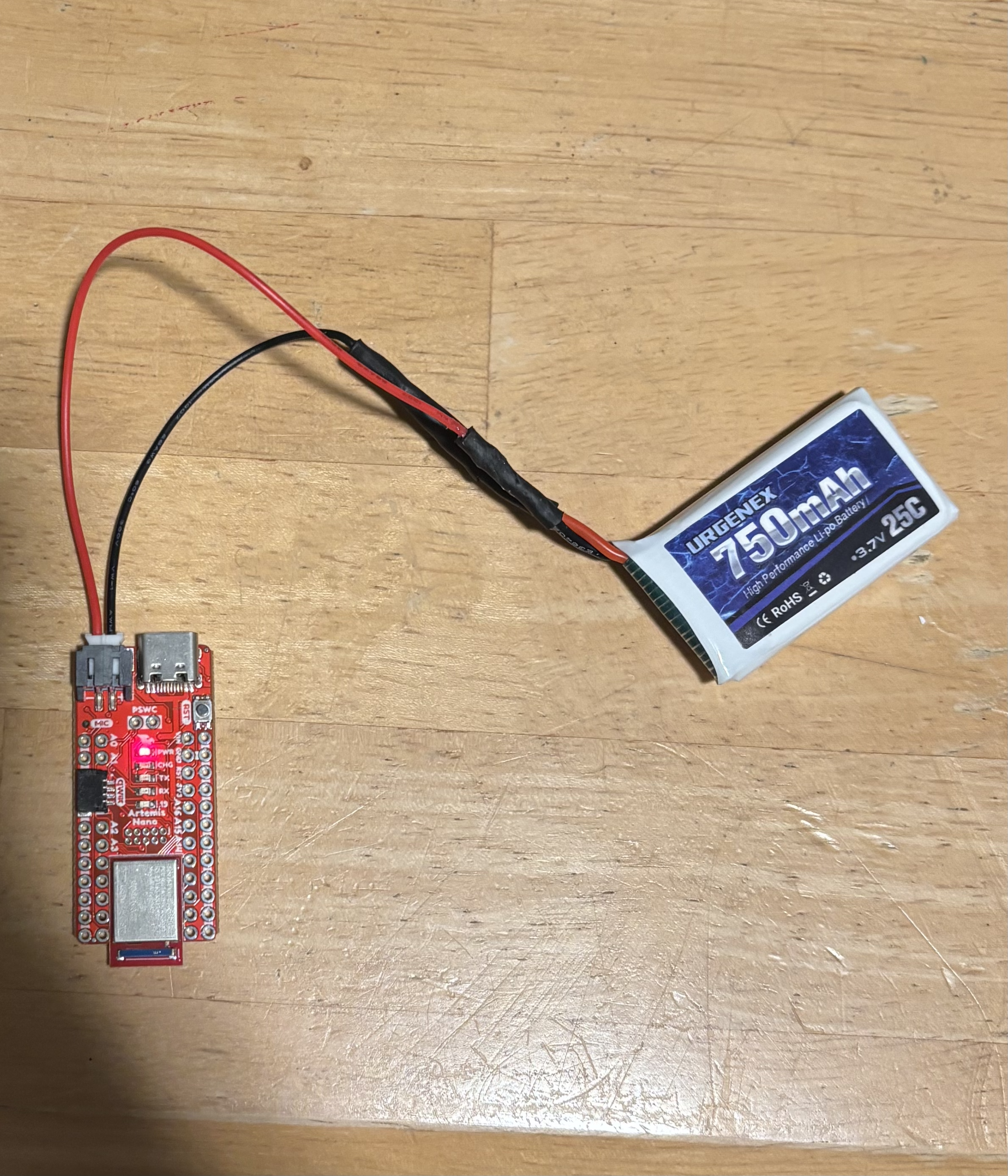
Battery
First, I soldered the battery wires to the JST jumper wires. I checked the polarity on the Artemis port to ensure that I was connecting the wires correctly, and then tested the battery by sending BLE data from the Arduino IDE to my computer (using previous lab code).
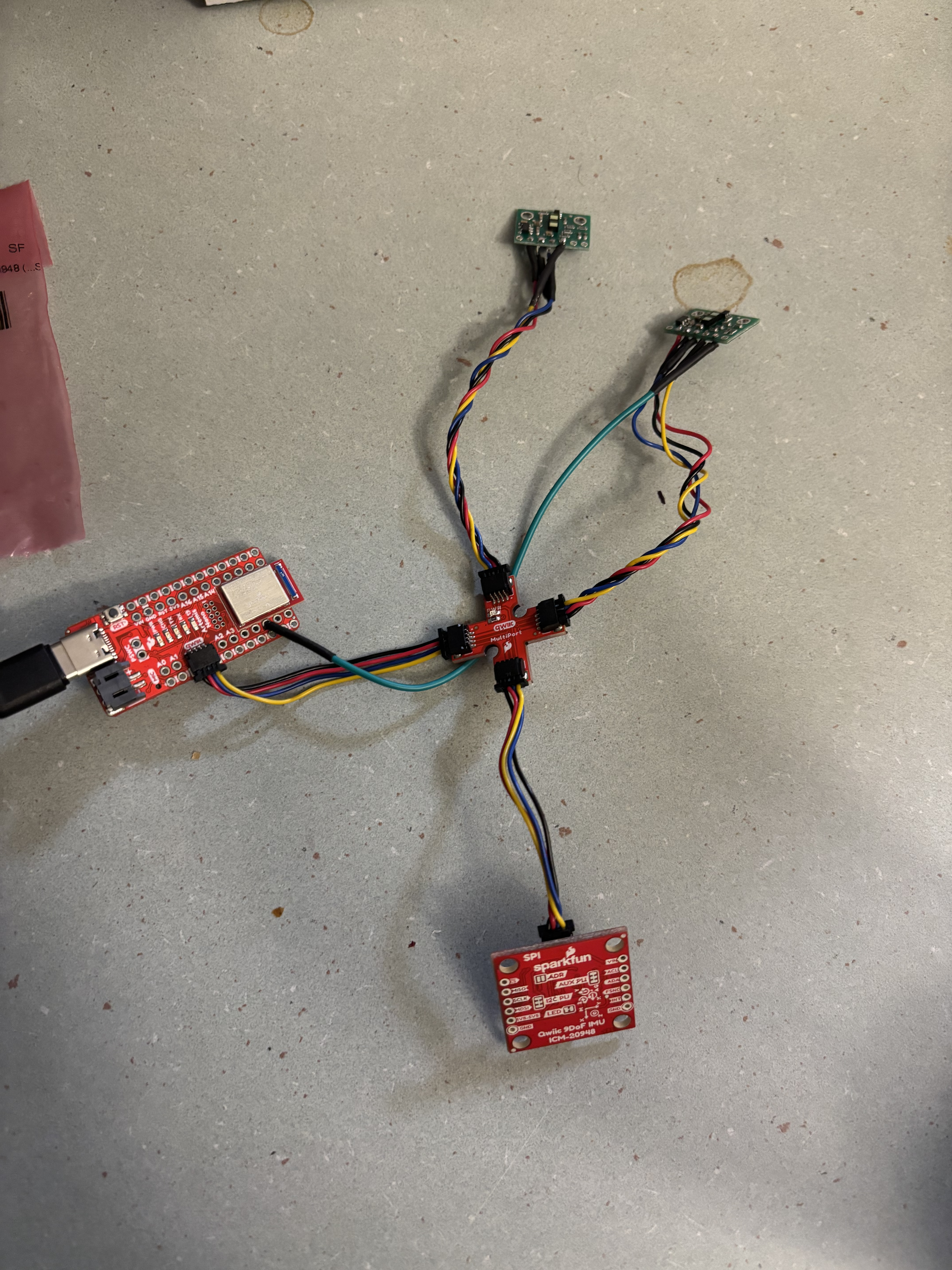
ToF Sensors
Following my wiring diagram plan, I soldered the ToF sensors to two QWIIC connectors. For the second sensor, I soldered a green wire from the XSHUT pin to pin 6 on the Artemis.
I2C Address
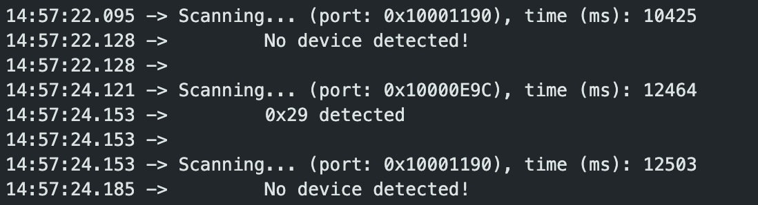
I installed the SparkFun VL53L1X 4m laser distance sensor library in Arduino IDE. Next, I ran Example05_Wire_I2C and found that the address was 0x29. This is different from the address listed in the datasheet, 0x52, because the address is shifted right one bit (0x52 >> 1 = 0x29) to account for the rightmost bit being used to identify if data is being read or written.
Three Modes
The ToF sensors have three modes: short, medium, and long. I looked into the pros and cons of each mode, and made a decision about which mode to use.
Discussion
Short: The short distance mode has a maximum distance of 1.3 meters and is the least susceptible to ambient light. Overall, this mode has greater accuracy and less noise than the other modes.
Long: The long distance mode has a maximum distance of 4 meters but is the most susceptible to ambient light.
Medium: This mode is only available with the Polulu VL53L1X Library, and therefore I did not take this mode into consideration. It has a detection distance between the short and long, and also has noise resistance between short and long.
I chose to use short mode for my robot because 1.3 meters is enough distance to detect obstacles, and the better resistance to noise will be greatly beneficial for when I run the car in different settings.
Testing
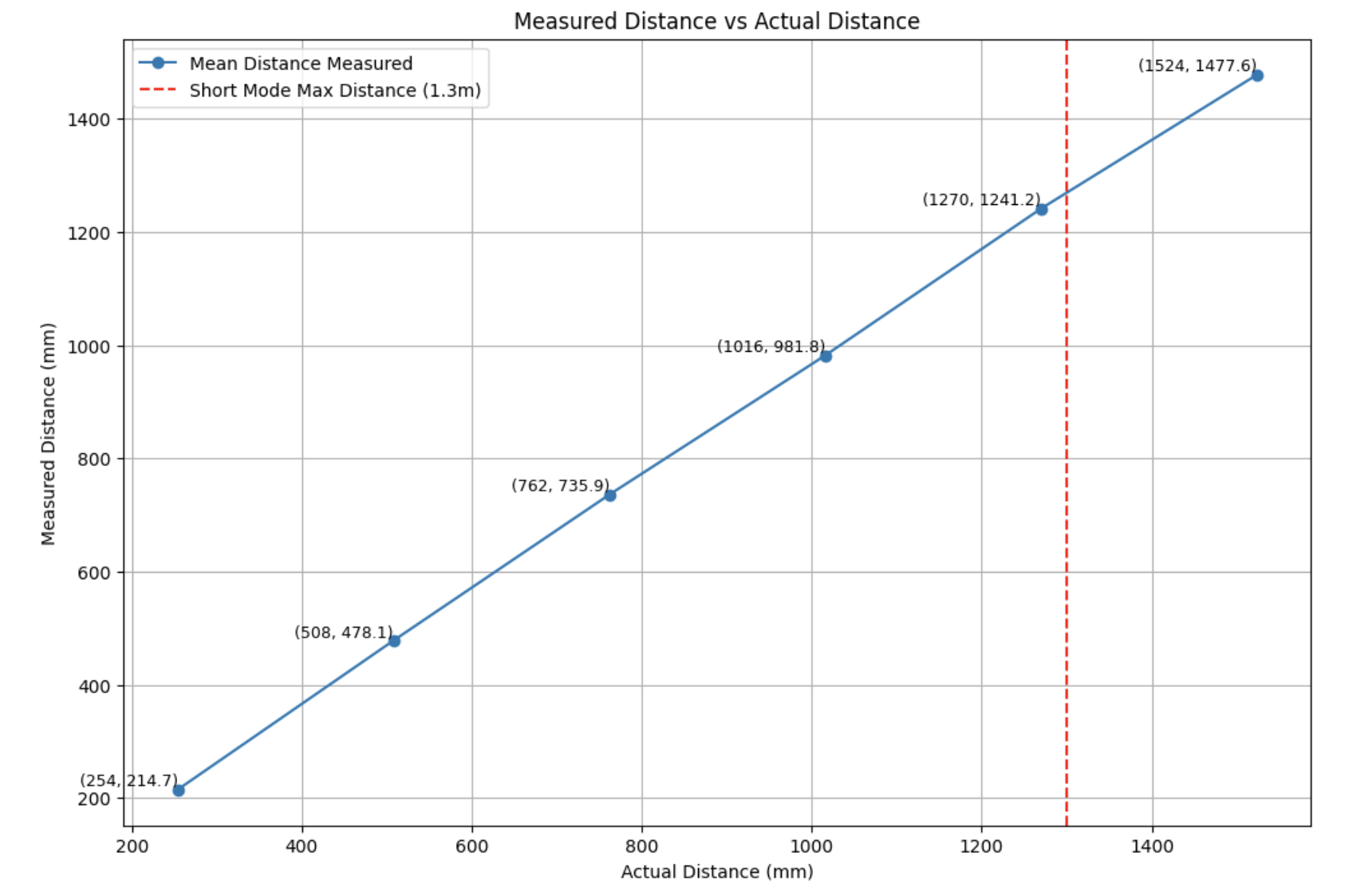
To test the ToF sensors at short mode, I taped one of the sensors flat on my laptop and used a tape measure to set up different distances from the wall. I decided to take 10 sensor measurements at six different distances:

10 in (254 mm)
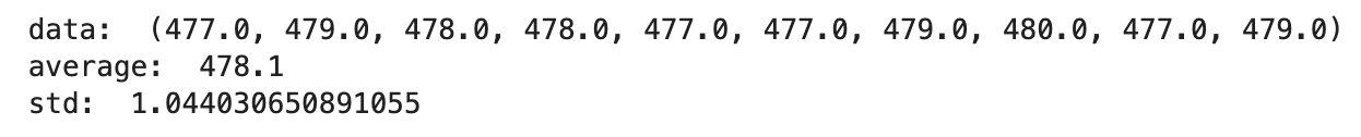
20 in (508 mm)
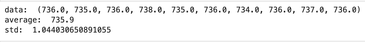
30 in (762 mm)

40 in (1016 mm)

50 in (1270 mm)
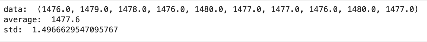
60 in (1524 mm)
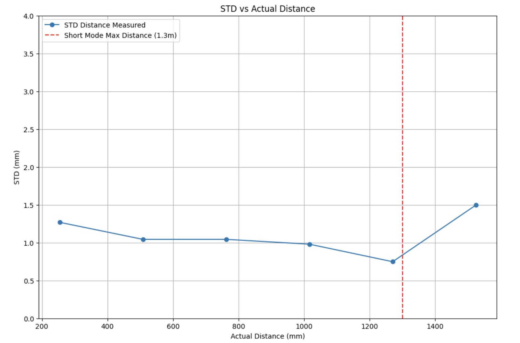
To check the accuracy of the sensors, I plotted the average values I calculated against the actual distances, shown below. From the plot, it can be seen that the measured distance has the greatest deviation from the actual distance at 1524 mm, which is outside of the short mode range. I also observed that the measured values were consistently less than the actual values, which could indicate a human error that remained throughout the data measurements. Because the experiment was manually set up, there was a lot of room for error, such as my laptop screen not being exactly aligned with the measuring tape distance due to a small angle deviation.
Next, in order to determine repeatability, I took the standard deviations of the measured sensor data and plotted it against the actual distances, shown in the figure below. Similar to the trend in the plotted average measurements, I observed that the standard deviation was its highest at 1524 mm, which is outside of the short mode range. The other standard deviation values remained close to 1.
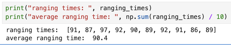
In order to measure ranging time, I took the start and end times at the beginning and end of each iteration of the data collection loop. From one test run, I noted that the ranging time hovered around the 90s (data shown below). These values were higher than I was expecting, which indicated that there was room for optimization within the data collection.
Two Sensors Working
The next task was to modify our code to collect data from both sensors instead of just one. To set this up, I switched between LOW and HIGH to set the address of the first sensor. The code to do this is shown below.
digitalWrite(XSHUT, LOW);
distanceSensor1.setI2CAddress(ADDRESS);
Serial.print("Distance Sensor 1 Address: 0x");
Serial.println(distanceSensor1.getI2CAddress(), HEX);

if (distanceSensor1.begin() != 0) // Begin returns 0 on a good init
{
    Serial.println("Sensor 1 failed to begin. Please check wiring. Freezing...");
    while (1)
        ;
}
distanceSensor1.setDistanceModeShort();
digitalWrite(XSHUT, HIGH);

Serial.print("Distance Sensor 2 Address: 0x");
Serial.println(distanceSensor2.getI2CAddress(), HEX);

if (distanceSensor2.begin() != 0) // Begin returns 0 on a good init
{
    Serial.println("Sensor 2 failed to begin. Please check wiring. Freezing...");
    while (1)
        ;
}
Serial.println("Sensors 1 and 2 online!");
distanceSensor2.setDistanceModeShort();
I also changed the code in the case statement in order to collect data from both sensors instead of just one. I then set up the second ToF sensor, also on my laptop, and collected data to ensure that they were functional. I did this by holding my laptop and rotating it and moving it around near a wall to get varied data.
Sensor Speed
The next task focused on optimizing our code to send data as fast as possible. To speed up my data collection loop, I moved the startRanding(), clearInterrupt(), and stopRanging() functions outside of the loop. My optimized code is shown below:
distanceSensor1.startRanging();
distanceSensor2.startRanging();

int st = millis();

for(int i = 0; i < array_size; i++)
{

    while (!distanceSensor1.checkForDataReady())    {
        delay(1);
    }
    distance1[i] = distanceSensor1.getDistance();

    while (!distanceSensor2.checkForDataReady())    {
        delay(1);
    }
    distance2[i] = distanceSensor2.getDistance();

    times[i] = millis();

}

int et = millis();

distanceSensor1.clearInterrupt();
distanceSensor1.stopRanging();
distanceSensor2.clearInterrupt();
distanceSensor2.stopRanging();
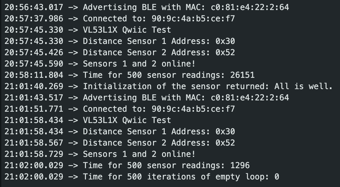
The variables st and et were used for me to check how quickly the loop executed. I ran this implementation, and also measured the time that an empty loop with the same amount of iterations took. As can be seen from the measurements in the photo below, it took 1296 ms to collect 500 sensor readings from each of the sensors (500 iterations of the loop, 1000 total messages). From this measurement, I calculated that it took an average of 2.592 ms per iteration of the loop. This is an immense improvement over the previously measured values of 90s. The increased speed is due to not having to continuously start, clear, and stop ranging.
Data Collection
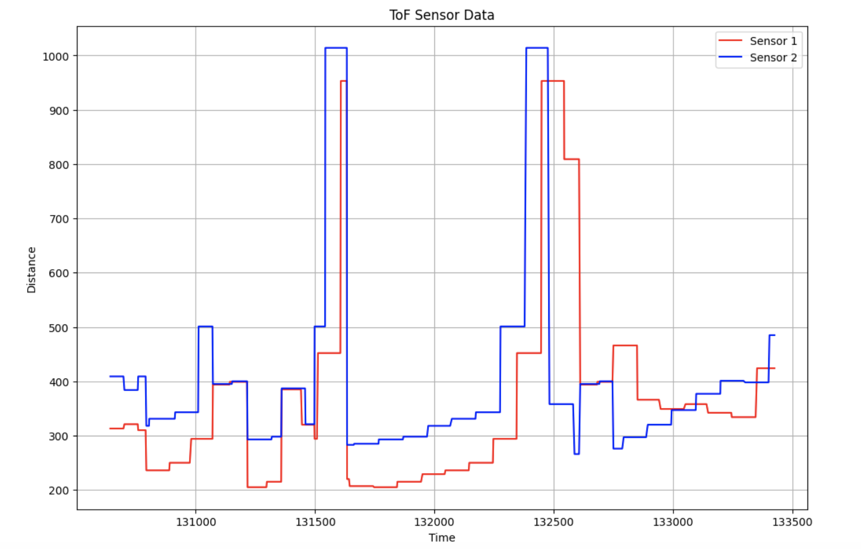
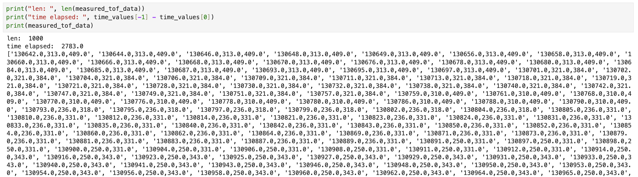
I used this optimized code to send over ToF sensor data to my python notebook and graphed that data over time. I used the same Python code logic as in Lab 2.
I also printed out the number of messages sent, as well as the time elapsed. These came out to be 1000 messages in 2783 ms, which is a sampling rate of 359.32 messages/second.
I then graphed IMU pitch data using my code from Lab 2, and also printed out all IMU data to analyze the speed.
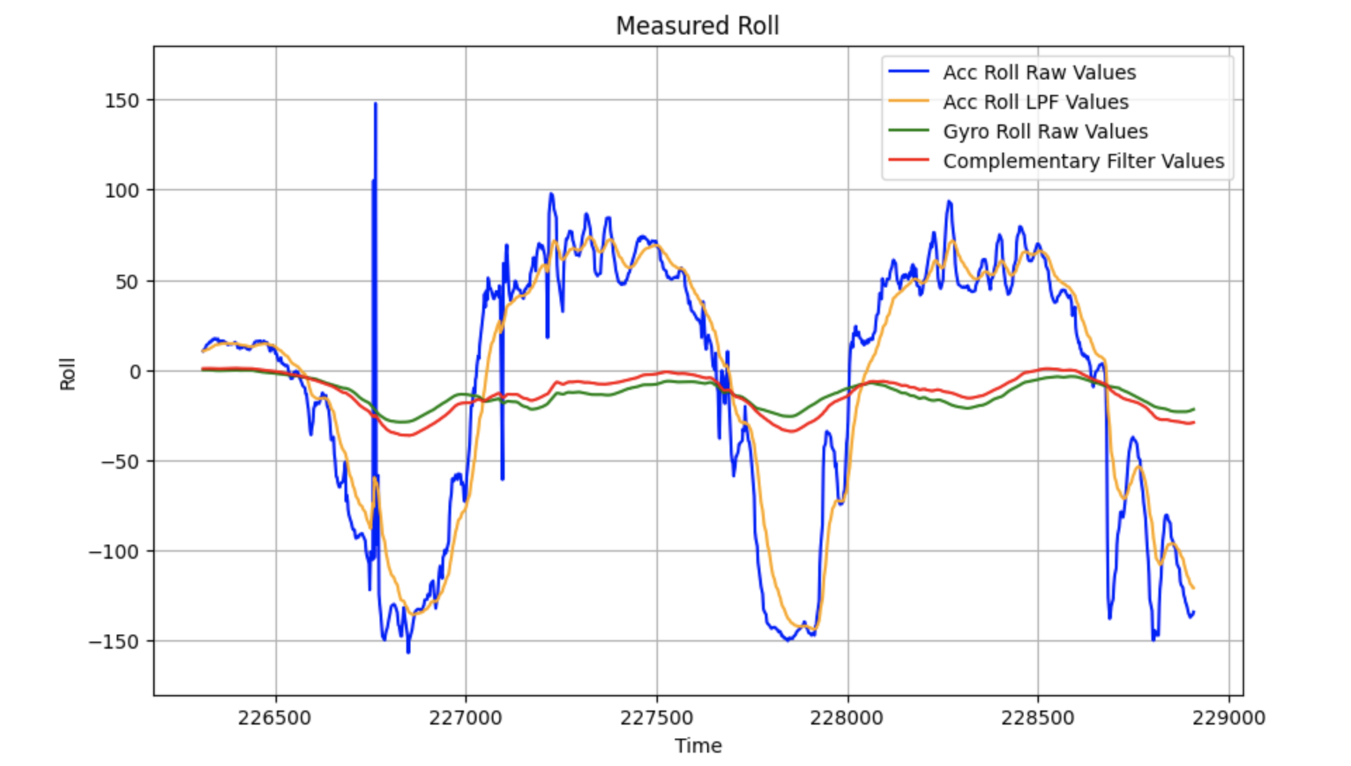
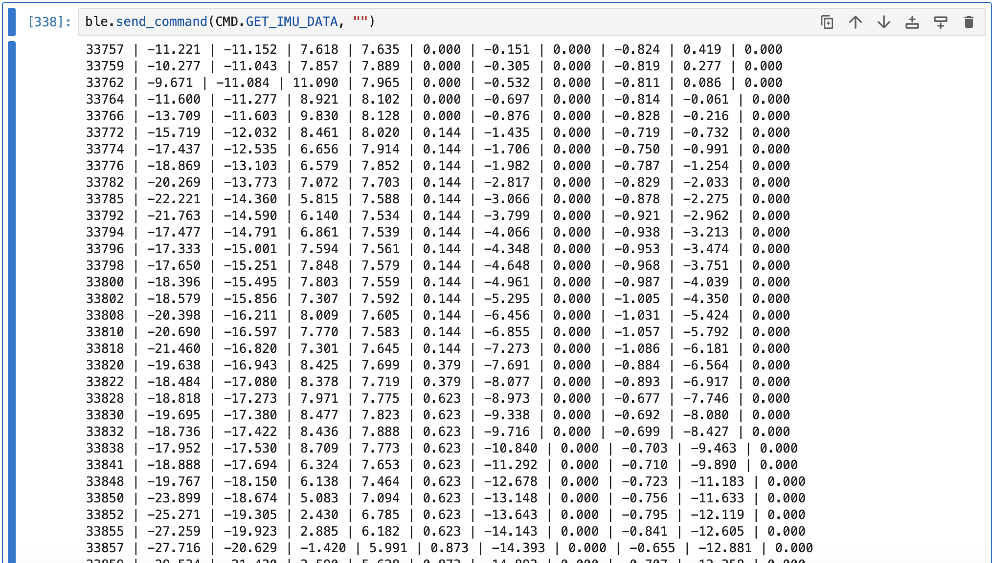
In comparison to collecting IMU data, the ToF sensors have a much faster sampling rate. Sending IMU data took 6.112 seconds for 1000 messages, which comes out to be a sampling rate of 163.61 messages/second. This could be due to the IMU sending over more data, as I had to send over measurements from the accelerometer, gyroscope, and also the filtered values.
References
I referenced Mikayla Lahr and Nila Narayan's past Lab 3 reports. Furthermore, I used the same hardware and corresponding set up as Sana Chawla (sc2347), but we each implemented our own software.